In a previous post, I speculated about a method of converting magnetometer readings to compass headings using affine transformations (specifically, three elemental rotations). In this followup, I’ll gather some real data, then see how those transformations actually work in the real world. Read on for details.
Update: This article is part of a larger series on building an AVR-based compass. You may be interested in the other articles in the series.
Gathering Test Data
When figuring out how to get real data, I decided on the following requirements:
- Use the same HMC5883L sensor I would be using in my compass project. (This excluded the possibility of using my Android tablet — which has a magnetometer build in — as a data source. This is something I did consider doing early on, and actually wrote some code for before deciding against it.)
- Use a “real” computer with local storage, network connectivity and easy debugging (as opposed to the AVR ATTiny85 I’m targeting for the compass project).
- Avoid buying any new hardware.
- Be able to rotate the entire test setup smoothly through at least a full circle on a fixed axis more-or-less normal to the ground.
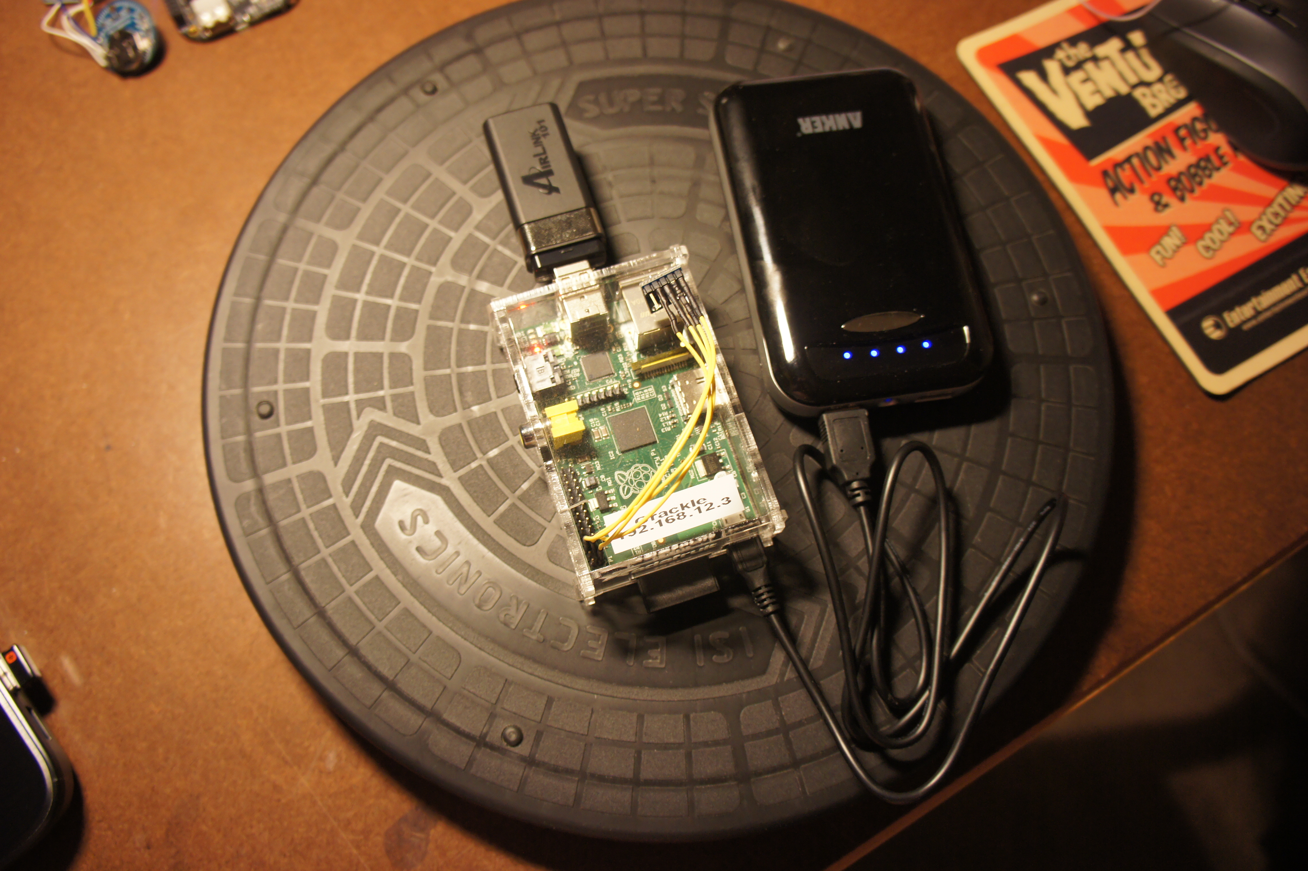 Fortunately I had a Raspberry Pi (original 256MB model B) sitting around that I could press into service. It was ideal as it had an I2C bus handy and would run fine on battery power. That, plus an ancient USB 802.11b wireless network card, a USB battery pack and a small “lazy susan” turntable, and I was in business.
You can see my experimental setup in the image to the right. Note how the sensor was placed as close as possible to the axis of rotation.
Wiring was very simple: I connected Pi pins 1 (3V3), 3 (I2C0 SDA), 5 (I2C0 SCL) and 6 (ground) to the corresponding pins on the sensor using Schmartboard jumpers. (I did not connect the DRDY pin on the sensor to anything.)
My Pi was set up to run Raspbian (a Debian derivative), so I had to do a little bit of work to get I2C set up. I followed the instructions from the Adafruit Learning System (ignoring the Python stuff and using the One True Editor instead of nano). I was able to see my sensor at address ‘1e’ on I2C bus 0. (Note that if you are using a newer Pi with 512MB of memory, you’ll see it on I2C bus 1 instead.)
Once the hardware was in place, I wrote a simple C program to initialize the sensor and gather data. The C API for doing I2C stuff in Linux is documented in the kernel tree, under Documentation/i2c/dev-interface. For the most part, I followed the example from the HMC5883L data sheet. I used the single measurement mode to simplify timing considerations for the non-real-time environment.
Note: As mentioned in the i2c/dev-interface docs, there are two copies of the i2c-dev.h header: one meant to be included from the kernel source, and another meant for userland applications. However, in Raspbian, the latter is not distributed with i2c-tools (as the dev-interface document claims). Instead, it lives in its own package: libi2c-dev. Make sure to install this!
The source for the data-gathering program is available for download: compass-read.tar.gz (8.6KB gzipped tarball).
My test protocol was to start the data collection program (from an SSH session on another network-connected computer) with my left hand while turning the turntable with my right. Once I’d made (approximately) a complete circle, I’d stop the collection program with ^C.
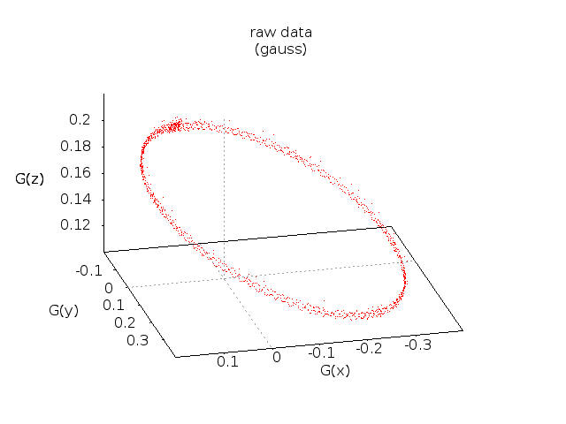
My results (on the first try!) were surprisingly good — see Figure 1 to the right. You can see the slight overlap between the start and end of the rotation in the slightly thicker part of the point cloud in the upper left. That looks like a nice ellipse in three dimensions, and is much less fuzzy that I expected. Promising.
My raw data are available for download as well: circle (40KB text file). The file format is one line per point, where lines are delimited by bare newlines (UNIX-style). Each line contains values for X, Y and Z (in Gauss), as human-readable floating point numbers separated by spaces.
Transforming Test Data
Now that I’ve got some real live data measured in a somewhat realistic test, let’s see what happens when we apply the transformations I described in my previous post. The source code for my test program is available for download: compass-tst1.tar.gz (14KB gzipped tarball).
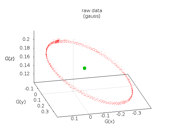
First, we find the center of the point cloud (by finding the average values for X, Y and Z across the entire set of points). That center is at {-0.054189, 0.078835, 0.162067}. See Figure 2.
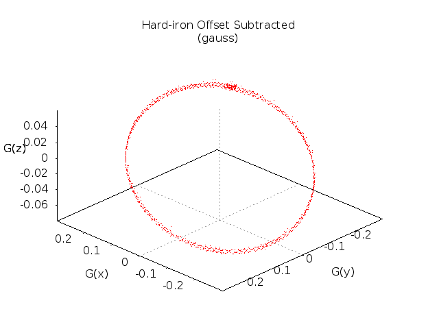
Next, translate the entire data set such that the center is at the origin. The results of this operation can be see in Figure 3:
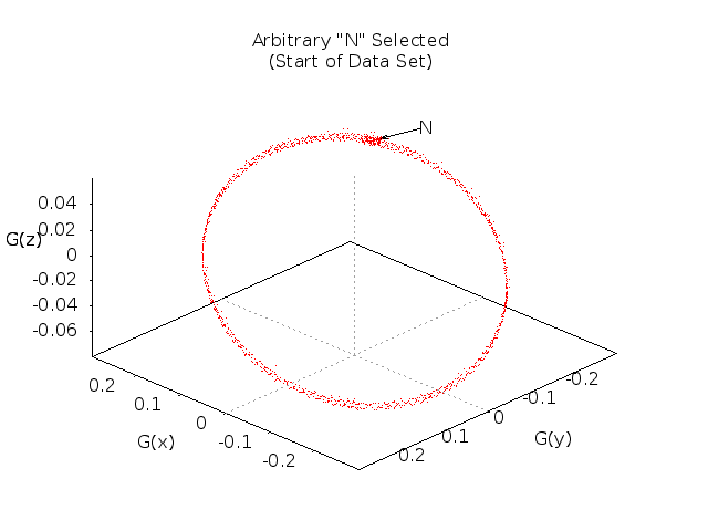
Designate the first point in the data set as ‘N’. This represents the requirement that the user orient the vehicle North prior to beginning the calibration process. See Figure 4:
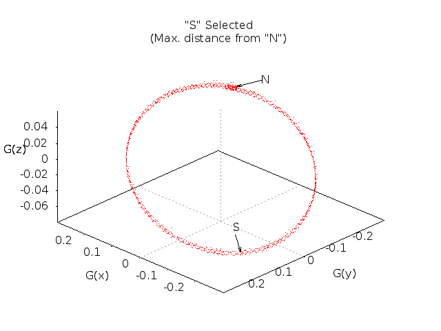
Find the point at the greatest distance from ‘N’ and designate it as ‘S’. (Note that while ‘N’ really is North by definition, ‘S’ is merely a point that’s generally near South in the case where there’s little soft-iron interference, and somewhere between 90° and 270° in the general case.) See Figure 5:
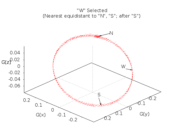
Find the point after ‘S’ in the data set which is most nearly equidistant to ‘N’ and ‘S’. Call this new point ‘W’. (This is not actually West. It will be if the data set is a perfect circle. In general, it can be any point which is somewhere on the Western half of the compass rose, and is not colinear with ‘N’ and the origin.) See Figure 6:
Something fortuitous has happened for the purposes of our example! See how ‘W’ is on the right-hand side of the circle? That’s because our sensor was hanging upside-down when we made the measurement. In other words, the graph is oriented so that we’re looking up through the bottom of the compass rose. That’s OK; our calibration process is designed to handle any orientation. It’ll get flipped over near the end of the process.
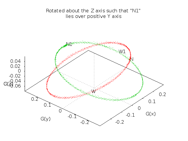
Rotate the entire data set about the Z axis such that point ‘N’ lies somewhere above, below or on the positive-Y part of the Y axis. (In other words, after the rotation, we want the X coordinate of ‘N’ to be 0 and the Y coordinate to be >0.) In Figure 7, the original point cloud is shown in red and the rotated point cloud in green:
The rotation involved is \(R_Z(\theta)\), in this case for \(\theta=146.88^\circ\):
\[R_Z(\theta)=\left[\begin{array}\cos\theta&-\sin\theta&0\\\sin\theta&\cos\theta&0\\0&0&1\end{array}\right]=\left[\begin{array}-0.838&-0.546&0.000\\0.546&-0.838&0.000\\0.000&0.000&1.000\end{array}\right]\]
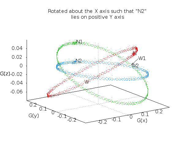
Now that ‘N’ is directly above or below (or on) the +Y half of the Y axis, we’ll rotate the whole data set again. This time, we rotate about the X axis to put ‘N’ directly on the Y axis (on the +Y side). In other words, we want the X and Z coordinates of ‘N’ to be zero, and the Y coordinate to be a positive value. Figure 8 shows the original point cloud in red, the cloud after the Z-axis rotation in green, and the point cloud after both rotations in blue.
The rotation involved is \(R_X(\theta)\), in this case for \(\theta=-11.39^\circ\):
\[R_X(\theta)=\left[\begin{array}{}1&0&0\\0&\cos\theta&-\sin\theta\\0&\sin\theta&\cos\theta\end{array}\right]=\left[\begin{array}{}1.000&0.000&0.000\\0.000&0.980&0.198\\0.000&-0.198&0.980\end{array}\right]\]
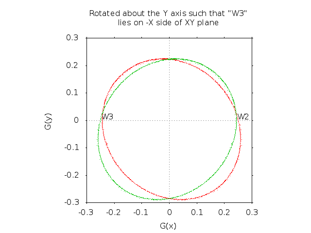
Finally, we rotate the entire cloud a third time. This third rotation is about the Y axis, and the angle is chosen such that after the rotation, ‘W’ lies on the XY plane, on the negative-X side of the Y axis. In other words, after the rotation, the Z coordinate of ‘W’ is zero and the X coordinate is negative.
For our particular set of test data, all the points happen to be very close to the XY plane after two rotations. (This is not the case in general.) After the third rotation, all the points are (by design, in the general case so long as the sensor readings are clean) near the XY plane. For clarity, I have plotted the results of the third rotation in only two dimension. In Figure 9, the data after two rotations is red and the data after three rotations is green. Notice that W is now on left side of the circle.
The rotation involved is \(R_Y(\theta)\), in this case for \(\theta=178.232^\circ\):
\[R_Y(\theta)=\left[\begin{array}{}\cos\theta&0&\sin\theta\\0&1&0\\-\sin\theta&0&\cos\theta\end{array}\right]=\left[\begin{array}-1.000&0.000&0.031\\0.000&1.000&0.000\\-0.031&0.000&-1.000\end{array}\right]\]
Now all of the points in the data cloud lie close to the XY plane in a rough circle centered on the origin where X=0, Y>0 is North and X<0, Y=0 is West. And, more importantly, we can compose the three rotations into a single rotation matrix. With a single translation (three numbers) and rotation (nine numbers), we can do the same thing to any future readings.
Once we have transformed a reading, it is trivial to find the angle made by unit North {0,1}, the origin {0,0} and the transformed reading. That angle is our compass bearing.
Future Work
The process presented here is useful as a proof of concept, but needs more work to be useful.
The most serious problem is that there’s nothing in my current code to deal with the discontinuity when point ‘N’ is very close to the Z axis. (I outlined dealing with this previously — we can just rotate about the X axis first, then Z. However, actually doing it is another matter.)
Obviously, I need to test on more than one data set, and try various different sensor orientations.
I should get some kind of angle-measurement tool and see how closely my calculated bearings correspond to actual rotation of the experimental platform.
It might be useful to add an additional scaling transformation to make the ellipse look more like a (unit) circle. However, until I compare measured vs. calculated bearings, that probably falls under the heading of “premature optimization”. (I need to remind myself that my goal here is to build a device that can read out the four cardinal directions — N E S W — and the four intercardinal — NE, SE, SW, NW. That only requires an angular accuracy of ±22.5°.)
Porting to the ATTiny85 will be challenging. I’ll have to use a different approach for finding ‘C’, ‘N’, ‘S’ and ‘W’ (where I keep a running average, and current best for the other points). Hopefully that plus coding for size rather than clarity will get the program to fit. If not, I may have to look at ditching the floating point library and going with fixed-point math instead, which is do-able but a lot of work.
Updated DGH 2014-03-04 to add note about libi2c-dev package for Raspbian. Thanks to WBD for catching the omission!
Updated DGH 2014-03-04 to add COPYING and README files to the example programs. Thanks to WBD a second time.
Good articles. They make a tough topic easy. Or perhaps all the other articles just made an easy topic difficult. Regardless I think that this will be helpful as I attempt to understand the mysteries of magnetometers.