I’m working on building a digital vehicle compass, using the Honeywell HMC5883L three-axis magnetometer as a sensor. Answering the question “Which compass direction am I facing?” from the raw sensor output data is somewhat more complicated that you might expect. This is especially true when using a microcontroller like the ATTiny85 with extremely limited memory. Read on for a discussion of the problems involved and my solutions.
Update: This article is part of a larger series on building an AVR-based compass. You may be interested in the other articles in the series.
Sensor Principles
To understand the problem, it is first necessary to understand a little bit about how the sensor works, in terms of what it’s actually sensing and how. The HMC5883L (790KB PDF datasheet) and similar sensors use three magnetoresistive elements. A magnetoresistive component is one which changes resistance in proportion to the strength of a magnetic field along its axis. (In this case, the material in question is a tiny strip of permalloy.) An important point to note is that each individual magnetoresistive element senses only the component of the magnetic field parallel to the element axis; it ignores field components orthogonal to the element axis. The three elements in the sensor package are oriented such that each one is orthogonal to the other two. In other words, one each in the X, Y and Z directions. Thus, when the sensor package is exposed to a magnetic field, the strength and direction of that field in three-dimensional space can be determined from the resistances exhibited by the three elements. (The elements are sufficiently small and close together that we can get away with assuming they all experience the same magnetic field.) The HMC5883L presents the magnetic field sensed as a vector of three signed 16-bit numbers (one for each axis). It also automatically compensates for any internal offset and temperature dependence of each element.
Update: The HMC5883L has a self-test mode which makes it possible to measure and compensate for temperature dependence. The application code still has to do so; the process is not automatic. Fortunately, a separate temperature sensor is not required.
Sensing Challenges
Specific obstacles to converting the field vector to a compass bearing include:
- We don’t know the orientation of the sensor axes relative to the horizontal plane (or gravity, if you prefer).
- We must compensate for hard-iron interference. This is a term of art which refers to the presence of permanent magnets in the vicinity of the sensor.
- We must compensate for soft-iron interference. This term refers to the proximity of materials with high magnetic permeability, which do not themselves have a magnetic field, but which attenuate the field we are trying to measure.
- We must compensate for magnetic declination. This is the variance between local direction of the Earth’s magnetic field and the direction of true (geographic) north. This difference can be quite large, for example from +20° to -20° within the continental U.S.
- The Earth’s magnetic field direction is not perfectly parallel to level ground. In other words, the field vector doesn’t point to (magnetic) north on the horizon, it points down into the ground on a shallow slope in a northerly direction.
There are other potential sources of error which, while real, I’m going to deliberately ignore either because their practical effect is minimal, or because compensating for them is intractably difficult, or both:
- The orientation of the sensor axes relative to the horizontal plane changes from moment to moment as the vehicle travels up and down slopes. We could compensate for this with an accelerometer, but it isn’t trivial to distinguish gravity from acceleration of the vehicle when things get bumpy.
- Local magnetic anomalies exist. I’m including in this broad category any hard- or soft-iron interferers which are not a fixed part of the vehicle. This can include interference from the surroundings or from time-variable sources within the vehicle itself (e.g., electric motors or small magnetic objects carried by passengers). Such anomalies will interfere with any magnetic compass system.
- Magnetic declination may change significantly if the vehicle travels a long distance. Compensating for this automatically would require a position reference and database, or an external direction reference.
- Magnetic declination changes significantly over time. However, the time scales involved in navigationally-significant changes are decades or centuries. It doesn’t seem burdensome to ask the user to re-calibrate more frequently than that.
Platform Challenges
As a self-imposed challenge, I’m trying to implement the compass on an extremely resource-limited embedded system: the Atmel ATTiny85, as present in the Adafruit Trinket. That means 512B (not MB, not KB) of RAM, 512B of EEPROM and around 2KB of usable program memory (after we allow space for the trinket bootloader, the display and I²C drivers and the floating-point math library). Floating-point math is probably not strictly necessary, but it makes things a lot easier. Using a tiny platform makes things fun and interesting because the obvious solutions to some of the problems involve collecting point clouds with hundreds or thousands of points, and using big programs like MATLAB (or at least libraries like LAPACK) for numerical analysis.
Assumptions
I’m going to make a few assumptions which I think are reasonable for the specific problem I’m trying to solve, but which may not be true in general:
- This compass system will not be used as a sole source of navigational information, or in any situation where the safety of life or property depends on correct operation.
- Accuracy within a few degrees is sufficient. A few heading updates per second is sufficient.
- The user will need to perform a calibration process when the compass system is first installed (and infrequently thereafter). The calibration process will involve facing the vehicle north (according to some independent external reference, signalling calibration start to the microcontroller (via a pushbutton input) then rotating the vehicle about the yaw axis +360° in a reasonable time frame (i.e., driving in a clockwise circle).
- During the calibration process, the turn rate will remain close to constant.
- The compass will remain at a fixed location and orientation relative to the vehicle during and after calibration.
- The user will re-calibrate when the vehicle moves far enough for the declination to change significantly.
- The vehicle remains at or near the surface of the Earth. (It’s a car, not a plane.)
- The vehicle remains within 45° of the horizontal plane. (If your car undergoes a full rotation about either the pitch or roll axis, you have much bigger problems than compass heading.)
- The compass system will not have constant electrical power. Calibration data must be stored in EEPROM to persist across power-off.
Numerical Model
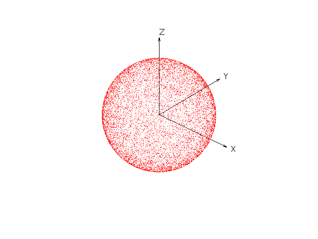
Consider the case where we take a hypothetical perfect sensor, and in the absence of any interference, rotate it at random (about all three axes) within a constant magnetic field. If we plotted the readings from this sensor as points in three-dimensional space, they’d appear on the surface of a sphere, centered at the origin and with a size proportional to the strength of the field. (See figure 1 at right; click for larger image.)
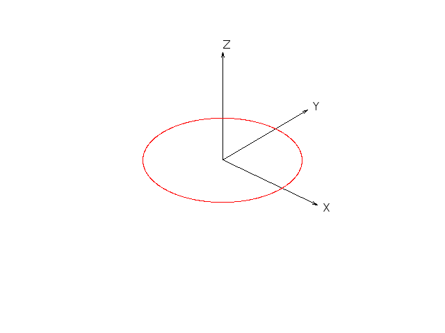
Now, let’s constrain the rotation to be about a single fixed axis. For the sake of example, we’ll use the Z axis. Now we get a circle in the XY plane, centered on the origin, with a radius proportional to the size of the field. See figure 2.
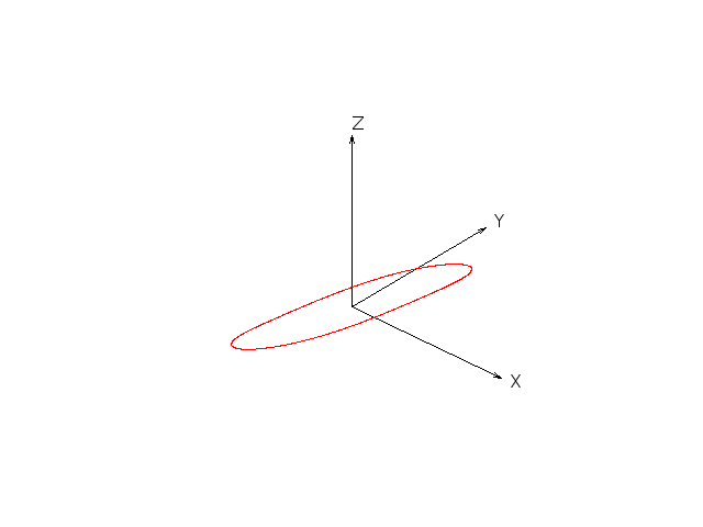
However, we don’t know in advance where the axis of rotation of our vehicle (yaw axis) is relative to any of the sensor axes, though we do know that they are fixed relative to one another. In our model, we still have a circle with the same center and radius, except now it’s tilted at an arbitrary angle. See figure 3. (Since the diagram is a 2D projection of a three-dimensional plot, it’s not completely clear. The circle in the figure isn’t on — or coplanar with — XY, XZ or YZ.)
There’s also hard-iron interference: sources of magnetism which are part of — and rotate with — the vehicle. In our model, this acts as an offset of arbitrary (but constant) distance and direction. We still have a circle with the same radius, but the center is no longer at the origin. Now the entire thing is shifted (in addition to being tilted). See figure 4.
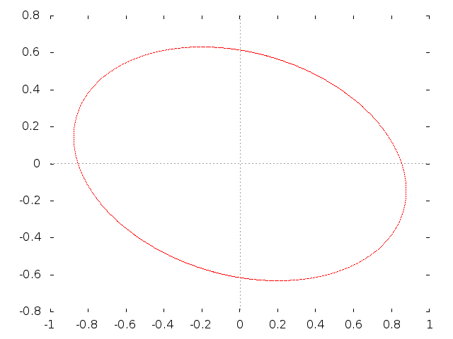
Soft-iron interference attenuates the measured field, and does so proportionally more in an arbitrary (but fixed) direction. Now our offset, tilted circle has been squashed into an ellipse (with a major axis that probably isn’t parallel to any of our coordinate axes). Figure 5 illustrates this effect (in two dimensions, with no tilt or offset, which will hopefully make it more clear).
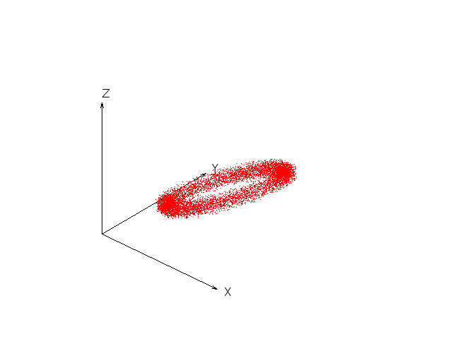
Finally, there’s noise (both from imperfections in the sensor, and magnetic anomalies in our environment). We’ll model this as a (hopefully, small) random offset in each point. Putting all the effects together, our perfect circle has become a tilted, shifted, fuzzy ellipse-like point cloud. See Figure 6.
That leaves us with two problems:
- Come up with a mapping from an arbitrary point in 3-space (which is hopefully somewhere on or near our fuzzy ring) to a scalar bearing (where geographic north is zero).
- During the calibration process, measure and quantify everything we need to know to know in order to perform the mapping in (1).
(And, of course, this must be done within the limitations of our computing platform.)
The Easy Way
If we know the centroid of our point cloud, we can subtract away the hard-iron interference, leaving the cloud centered on the origin. Now we can treat (adjusted) readings as vectors from the origin to their coordinates. If we have a reading corresponding to north (call it \(\vec{N}\)) and another reading \(\vec{A}\), we can find the angle between them using the dot product:
\[\begin{align}\vec{N}\cdot\vec{A}&=\|\vec{N}\|\|\vec{A}\|\cos\theta\\\nonumber\\\theta&=\cos^{-1}\frac{\vec{N}\cdot\vec{A}}{\|\vec{N}\|\|\vec{A}\|}\end{align}\]
This should give a “good enough” heading for some applications, and is relatively easy. If it works for what you’re doing: great! However, I’m going to go on to explore a more complicated solution, for three reasons:
- The above doesn’t give you a way to determine the correct sign of theta. Maybe the user mounted the system upside-down?
- You can’t detect readings which are significantly outside the plane of the point cloud acquired during calibration. Such points represent transient magnetic anomalies, and it would be nice to be able to discard them or warn the user rather than simply displaying a false heading.
- It requires a bit of extra computation for each reading (relative to other methods). There are ten multiplications, one division, two square roots and a trig function:
Let \(\vec{N}=\begin{bmatrix}x_N\\y_N\\z_N\end{bmatrix}\) and \(\vec{A}=\begin{bmatrix}x_A\\y_A\\z_A\end{bmatrix}\). Then:
\[\begin{align}\|\vec{N}\|&=\sqrt{x_N^2+y_N^2+z_N^2}\\\|\vec{A}\|&=\sqrt{x_A^2+y_A^2+z_A^2}\\\vec{N}\cdot\vec{A}&=x_{N}x_A+y_{N}y_A+z_{N}z_A\\\nonumber\\\theta&=\cos^{-1}\frac{x_{N}x_A+y_{N}y_A+z_{N}z_A}{\sqrt{x_N^2+y_N^2+z_N^2}\sqrt{x_A^2+y_A^2+z_A^2}}\end{align}\]
I think I’ve found another method that involves more complexity at calibration time, but somewhat simplifies the process of turning subsequent readings into headings.
My Proposed Solution
Calibration
During the calibration process, I wish to learn the (approximate) location (in terms of X, Y and Z coordinates) of four specific points:
- The reading that corresponds to the vehicle facing geographic north: \(N\)
- The first reading which is at a maximum distance from \(N\): \(M\)
- The reading obtained after finding \(M\) which is the closest to being equidistant from \(N\) and \(M\): \(W\mid\|\overrightarrow{WN}\|\approx\|\overrightarrow{WM}\|\)
- The position that corresponds to the constant offset from hard-iron interference (i.e., the centroid of the point cloud): \(C\)
Finding \(N\) is trivial, since we require that the user start the calibration process with the vehicle facing north (and signal us when calibration should begin). So, we simply take a reading at the start of the calibration process and declare it to represent geographic north by definition.
For \(M\), we will continuously take readings throughout the calibration process. (By “continuously” I mean as fast as the sensor and microcontroller can reliably handle. That should be at least a few tens of points per second.) We will remember the reading that represents the first maximum in linear distance from the “north” point we found previously.
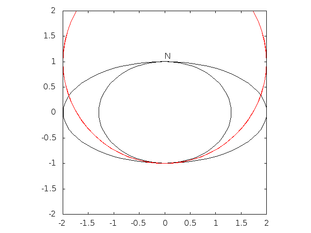
For ellipses of low eccentricity, the maximum distance is on the opposite side (“south”). For ellipses of higher eccentricity (i.e., in the presence of stronger soft-iron interference), there are two maxima: one in the southeast quadrant and one in the southwest. (For the degenerate case where the minor axis is zero and the ellipse is a line segment, they are east and west.) In Figure 7 (right) the red circle represents a fixed distance from north. The smaller (less eccentric) ellipse touches the circle at exactly south. The larger (more eccentric) ellipse is outside the circle in the southeast and southwest.
In the above diagram, north happens to be placed on the minor axis of the ellipse. This is not necessarily the case in general.
Where \(a\) and \(b\) are the lengths of the major and minor axes, the parametric equations for an ellipse are: \(X(t)=a\cos t; Y(t)=b\sin t\). This gives us the following equation for distance between two points on the ellipse in the general case:
\[\begin{align}d&=\sqrt{(X(t_1) – X(t_2))^2 + (Y(t_1) – Y(t_2))^2}\\&=\sqrt{(a\cos t_1 – a\cos t_2)^2 + (b\sin t_1 – b\sin t_2)^2}\\&=\sqrt{a^2(\cos^2 t_1 -2\cos t_1 \cos t_2 + \cos^2 t_2) + b^2(\sin^2 t_1 – 2\sin t_1\sin t_2 + \sin^2 t_2)}\\&=\sqrt{a^2(1-\sin^2 t_1 – 2\cos t_1 \cos t_2 + 1 – \sin^2 t_2) + b^2(\sin^2 t_1 – 2\sin t_1\sin t_2 + \sin^2 t_2)}\\&=\sqrt{2a^2-a^2\sin^2 t_1 – a^2\sin^2 t_2 -2a^2cos t_1 \cos t_2 + b^2\sin^2 t_1 + b^2\sin^2 t_2 -2b^2\sin t_1 \sin t_2}\\&=\sqrt{2a^2+(b^2-a^2)\sin^2 t_1 +(b^2-a^2)\sin^2 t_2 -2a^2\cos t_1 \cos t_2 – 2b^2\sin t_1 \sin t_2}\end{align}\]
For fixed values of \(a\), \(b\) and \(t_1\), we are trying to find the maximum value of \(d\). We can ignore the terms that are constant (i.e., that depend only the fixed values) and maximize:
\[x=(b^2-a^2)\sin^2 t_2 – 2a^2\cos t_1 \cos t_2 – 2b^2\sin t_1 \sin t_2\]
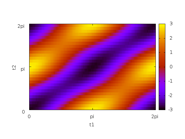
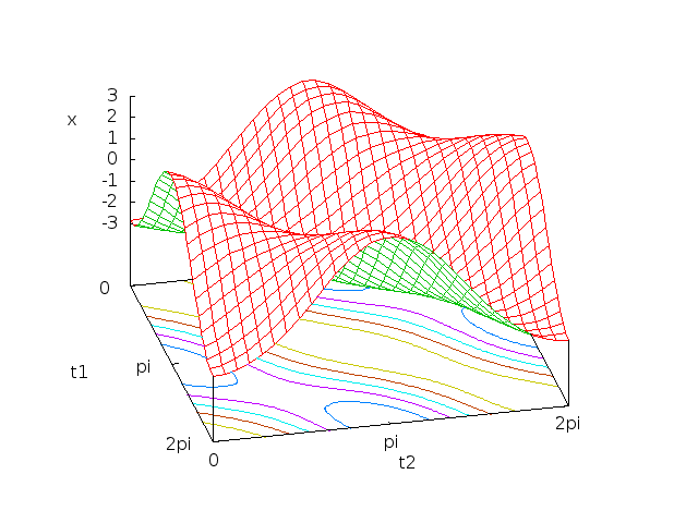
When eccentricity is low, the maximum is where \(t_1 – t_2 = \pm\pi\). Figures 8a and 8b illustrate the value of \(x\) for various values of \(t_1,t_2\) for the case where \(b=1\) and \(a=1.2\). For any fixed value of \(t_1\) there is a value of \(t_2\) where \(x\) is maximum, and it’s always a half-circle (\(\pi\) radians) away:
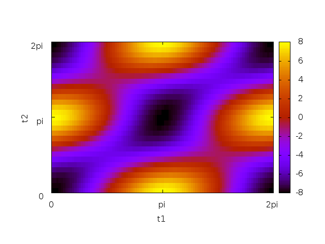
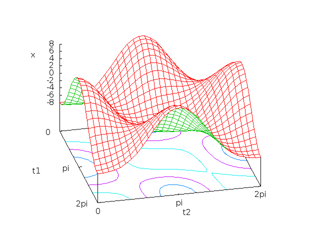
Now consider the case where the eccentricity is larger. Figures 9a and 9b illustrate what happens when \(b=1\) and \(a=2\). When \(t_1\) is close to the minor axis, there are two distinct maxima. As \(t_1\) draw closer to the major axis, there’s a single maximum half a circle away (as in the low-eccentricity case).
The point of all that is that the general rule on which we depend (the first or only maximum is in the southeast quadrant when \(t_1\) is defined to be north) still applies.
As a practical matter, to ensure we find the first (southeast) maximum in the highly eccentric case, when considering a new maximum, we will require that it exceed the old favorite by a positive value of a function that increases monotonically with distance between the new candidate and the old favorite.
Point \(W\) — the reading found after \(M\) which is most nearly equidistant from \(N\) and \(M\) — is trivial. For each new reading, we measure the distances to \(N\) and \(M\), take the difference, and if it’s the smallest found so far, that reading is our new candidate for \(W\).
In some ways, point \(C\) (the centroid of the point cloud) is most problematic. If I had lots of memory and computing power to spare, I’d probably do something like: collect all the points, discard outliers, construct the convex hull of the set of remaining points, then find the centroid of that volume. On a microcontroller, the best I have come up with so far is to average the readings across the entire calibration process. (This is the reason I stated the assumption that the turn rate during the calibration process remains close to constant. Large variations would mean that two equiangular arcs of our ellipse would contain very different numbers of readings, skewing the average toward the side with more readings.)
The calibration process will be considered complete when \(M\) has been found and the distance between the current reading and \(N\) becomes small relative to \(\|\overrightarrow{NM}\|\).
Tranforms
Given point \(C\), it’s easy to construct a linear translation that puts it at the origin. We just subtract the Cartesian coordinates of \(C\) from all the points we are working with. As a practical matter, we’ll do this first to simplify the remaining work.
We now have a point cloud with its center at the origin. Let \(\vec{N}\) and \(\vec{W}\) be vectors from the (new) origin to the (adjusted) positions of points \(N\) and \(W\) respectively.
We wish to construct a rotation such that \(N\) (“north”) lies along the positive Y axis, and \(W\) lies on the negative-X side of the XY plane. We can do this in three elemental rotations:
- Rotate about the Z axis such that the X coordinate of \(\vec{N}\) is zero and the Y coordinate is positive. In other words, we’re making “north” sit somewhere directly above, below or on the positive Y axis. Let \(R_1\) be the matrix for this rotation, and let \(\vec{N_1}=R_1\vec{N}\) and \(\vec{W_1}=R_1\vec{W}\).
- Rotate about the X axis such that the Z coordinate of \(\vec{ N_1}\) is zero and the Y coordinate remains positive. Call the matrix for this rotation \(R_2\). So, after the first two rotations, \(\vec{N_2}=R_2\vec{N_1}\) lies on the positive Y axis. Let \(\vec{W_2}=R_2\vec{W_1}\).
- Rotate about the Y axis such that the Z coordinate of \(\vec{W}\) is zero and the X coordinate is negative. (Since \(\vec{N_2}\) already lies on the axis of rotation, it does not move as a result of this step.) Let this rotation be \(R_3\), so \(\vec{N_3}=R_3\vec{N_2}\) and \(\vec{W_3}=R_3\vec{W_2}\).
Note: If \(N\) lies on the Z axis before we start, then step (1) cannot be carried out unambiguously — any rotation about the Z axis leaves \(N\) above or below the Y axis. (And, as a practical matter, if \(N\) is very close to the Z axis, then approximating step (1) using float-point math on a computer involves a potentially large degree of numerical error.) To remedy this, we can just swap steps (1) and (2) if \(N\) is very close to the Z axis. (Because of how we performed the calibration process, \(N\) and \(W\) cannot be colinear with the origin. Thus, at most one of \(N\) and \(W\) can be close to the Z axis.)
So:
\[R_1\vec{N}=R_Z(\theta_1)\vec{N}=\begin{bmatrix}\cos\theta_1&-\sin\theta_1&0\\\sin\theta_1&\cos\theta_1&0\\0&0&1\end{bmatrix}\begin{bmatrix}x_N\\y_N\\z_N\end{bmatrix}=\begin{bmatrix}x_N\cos\theta_1-y_N\sin\theta_1\\x_N\sin\theta_1+y_N\cos\theta_1\\z_N\end{bmatrix}=\begin{bmatrix}0\\\gt 0\\z_N\end{bmatrix}\]
That means that to find \(R_1\) we just need to find \(\theta_1\) such that \(x_N\cos\theta_1= y_N\sin\theta_1\) and \(x_N\sin\theta_1+y_N\cos\theta_1\gt 0\).
We know that:
\[a\sin\theta+b\cos\theta=\sqrt{a^2+b^2}\sin(\theta+\psi) \; \mbox{where }\; \psi=\tan^{-1}\frac{b}{a}+\begin{cases}0&\mbox{if } a\ge 0\\\pi&\mbox{if } a\lt 0\end{cases}\]
Thus:
\[\begin{align}0&=y_N\sin\theta_1+(-x_N)\cos\theta_1\\&=\sqrt{y^2_N+x^2_N}\sin(\theta_1+\psi)\end{align}\]
We are given that \(N\) does not lie on the Z axis, so at least one of \(x_N\) and \(y_N\) is non-zero. Therefore, \(\sqrt{y^2_N+x^2_N}\gt 0\) so we are just trying to solve \(\sin(\theta_1+\psi)=0\). Since \(\sin(x+\pi)=\sin x\) for all real \(x\), we can solve for \(\theta_1\):
\[\sin(\theta_1+\tan^{-1}\frac{-x_N}{y_N})=0\\\theta_1+\tan^{-1}\frac{-x_N}{y_N}=n\pi \; \mbox{for } \; n=0,1\\\theta_1=n\pi – \tan^{-1}\frac{-x_N}{y_N} \; \mbox{for } \; n=0,1\]
That yields two distinct solutions. However, only one of them satisfies the requirement that \(\vec{N_1}\) lies above the positive Y axis.
Now that we know the value of \(\theta_1\), we can populate the matrix \(R_1\) with real numbers.
Using a similar process, we can construct constant-valued matrices \(R_2\) and \(R_3\).
Since \(B(A\vec{x})=(BA)\vec{x}\), we can compose the three elemental rotations into a single transformation by multiplying the matrices such that \(R\vec{x}=R_3(R_2(R_1\vec{x})))=(R_{3}R_{2}R_1)\vec{x}\).
It’s tempting to toss our original translation (to make \(C\) the new origin) into the mix. We can do so easily enough using homogeneous coordinates, giving each matrix an extra row and column, which are all-zero save for a 1 in the lower right). So, in our original as-measured coordinate system:
\[\mbox{If } C=\begin{bmatrix}x_C\\y_C\\z_C\\1\end{bmatrix} \; \mbox{then } \; R_T=\begin{bmatrix}1&0&0&-x_C\\0&1&0&-y_C\\0&0&1&-z_C\\0&0&0&1\end{bmatrix}\]
That gives us a four-dimensional linear transformation matrix \(T=R_{3}R_{2}R_{1}R_T\) such that we can project any measured reading onto the XY plane. (where the origin is magnetic zero and positive Y is north), and (optionally) a Z coordinate that we can use to help detect anomalous readings. The bearing we want is then just \(\theta=\tan^{-1}(x/y)\).
However, it turns out to be computationally less expensive to do the translation as three subtractions up-front. Then it requires only six multiplications (instead of eight) to get our transformed X and Y coordinates. (If we want Z as well, it takes nine multiplications instead of twelve.)
Since we only need to calculate the X and Y (and maybe Z) coordinates, we need only store nine (or twelve) floating point numbers in EEPROM to represent the calibration data. Calculation of a bearing requires six (or nine) multiplications, one division and one trig function.
Room for Improvements
- I’m not that great at math to begin with, and haven’t messed with linear algebra in probably 20 years. There are likely errors, and I’ve almost certainly completely missed easier/better ways of doing the same thing.
- Seriously: Don’t use this to sail out of sight of land (or base a product on it) without a lot of verification first. I haven’t even tried it on real data yet!
- There should be another (scaling) transformation in there to un-squash the ellipse. The error isn’t huge unless the eccentricity gets big, but still…
- While we’re at it, the scaling transformation should also put our readings somewhere close to the unit circle. That makes anomaly detection easier, for one thing.
- Finding the centroid is a kluge.
There’s no code or real data sets yet. Working on it, promise!There is now a followup article with real data and working code.
Comments and corrections always welcome.
Updated DGH 2014-03-03 to add link to second article with real data and working code.
Updated DGH 2014-04-28 to add correction regarding temperature compensation.
Updated DGH 2019-10-08 to fix problem with equations not rendering properly. (The LaTeX plugin I was using didn’t work with the latest WordPress update.)
Hi, It’s not exactly a comment but a help request. I intend to construct a sensor using 3 of the same sensor HCM5883L, positioned near each other, at 120º apart. what I need is a algorithm or sample code to detect the direction of circular moving small magnet, like a moving pendulum .
I’ve made one using 5 hall’s sensor using 5 channel ADC in MBED processor.
its worked, but its seems no so good. I think that the HCM5883L Will give more information and less wires hook-up (I2C).
Thanks for any reply: Best Regards: Dorisvaldo
Hello, Dorisvaldo.
That sounds like a cool project. If your sensors are fixed in place, I’d suggest starting by taking a reading (from each sensor) without the moving magnet. That’ll give you a baseline for the Earth’s magnetic field plus local interference, which should be a (roughly) constant 3-vector. You can subtract that out of all your subsequent readings to get just the field vector due to your moving magnet.
The simplest approach from there is probably to just look at the magnitude of the remaining vector from each of the three sensors. If you know how strong it is when the moving magnet is right over the sensor, and how strong it is when the moving magnet is far away, you should be able to triangulate and get a rough position.
Using the direction is hard, because the field lines from your moving magnet are most likely a funny shape like a squashed torus. Modelling this mathematically is certainly possible, but way beyond my skill.
Hello, i was wondering how you got the ATtiny85 to “talk” til the HMC5883L?
I’m working on a project where i’m using a HMC5883L to detect when a car is passing by, and it works with arduino Uno and Nano, but i can’t get the ATtiny85 to program.
Thanks :)
keep in mind that “north” changes as much as 30 degrees depending where on earth you are (called declination – see http://www.magnetic-declination.com/), and that it’s not horizontal to the ground either (confusingly, called “inclination” – see https://physics.stackexchange.com/questions/283761/if-you-hold-a-compass-needle-vertical-does-it-point-down-or-up-differently-on-wh/283782
Chris @#4: Good information about declination and inclination.
The code for this project includes a calibration step where you start facing (local, geographic) north, then turn in a full circle (on the horizontal plane). This produces a transformation matrix that compensates for both declination and inclination.
If you move far enough for there to be a significant change in declination (or inclination), you have to repeat the calibration process to get accurate readings.
Another cool thing is that the magnetic vector at a given point on the earth’s surface changes over time. (Very gradually, but in human-scale time rather than geological scale. )